Autograd Engine & Neural Network Classifier
A from-scratch implementation of automatic differentiation and backpropagation, the core engine behind modern deep learning. Includes a scalar-valued autograd engine, linear layer, softmax cross-entropy loss, and a gradient descent training loop that achieves 99% accuracy on a 4-class 2D classification task.
Autograd Engine & Neural Network Classifier
Overview
A from-scratch implementation of automatic differentiation and backpropagation, the core engine behind modern deep learning. Includes a scalar-valued autograd engine, linear layer, softmax cross-entropy loss, and a gradient descent training loop that achieves 99% accuracy on a 4-class 2D classification task.
Project Overview
Automatic differentiation (autograd) is the foundation of every modern neural network framework. PyTorch, TensorFlow, and JAX all rely on it to compute gradients efficiently. This project builds a scalar-valued autograd engine entirely from scratch in Python, using nothing beyond NumPy. The goal was to deeply understand what happens beneath the abstractions of these frameworks by implementing every piece by hand.
The engine works by wrapping every number in the computation inside a Value object. Whenever two Value objects interact through an arithmetic operation (addition, multiplication, exponentiation, etc.), the engine automatically records that operation and creates a link between the input nodes and the output node. This process builds a dynamic computational graph as the computation unfolds. Each node in the graph stores its numerical result (the forward pass value) and a small function called _backward that knows how to compute the local gradient for that specific operation.
Once the full forward computation is complete, calling .backward() on the final output node walks the entire graph in reverse. It performs a topological sort to determine the correct order of traversal, then applies the chain rule at every node, multiplying the upstream gradient by the local gradient and accumulating the result into each input node’s .grad attribute. By the time this reverse pass finishes, every leaf variable in the graph (weights, inputs, biases) has its gradient fully computed.
The computational graph below shows this process in action for the function f = σ(w₁x₁ + w₂x₂) + 0.5(w₁² + w₂²), which combines a sigmoid neuron with L2 weight regularization. The green boxes show each node’s forward-pass data value, and the blue ellipses show the gradient computed during the backward pass. The orange circles represent the operations (multiply, add, exp, power) that connect the nodes together.
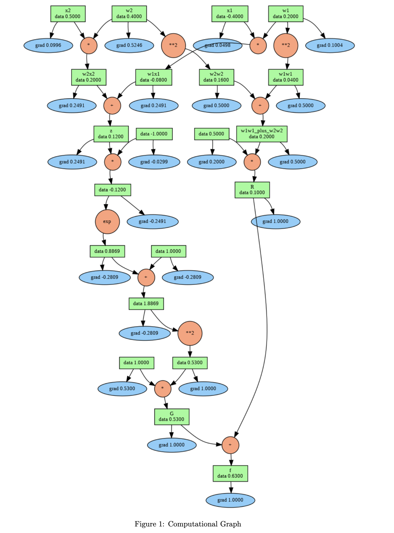 Figure 1: Computational graph for f = σ(w₁x₁ + w₂x₂) + 0.5(w₁² + w₂²) with w₁ = 0.2, w₂ = 0.4, x₁ = -0.4, x₂ = 0.5. Green boxes display forward-pass values. Blue ellipses display gradients computed via backpropagation. Orange circles represent operations.
After building and validating the autograd engine on this example, I used it to construct and train a linear neural network classifier on a 2D dataset with 4 classes and 100 samples. The model consists of a single LinearLayer(2, 4) followed by softmax and cross-entropy loss. Training with vanilla gradient descent at a learning rate of 1.0 converges to 99% accuracy within 500 iterations.
How It Works
The Value Class
The Value class is the core primitive of the engine. It wraps a single floating-point number and carries three additional pieces of state: a grad field (initialized to zero) that accumulates the gradient during backpropagation, a _prev set that tracks which Value nodes were used to produce this one, and a _backward closure that encodes the local gradient rule for the operation that created this node.
When you write something like c = a + b where a and b are both Value objects, the __add__ method creates a new Value with data = a.data + b.data, records (a, b) as its children, and attaches a _backward function that says “when I receive a gradient from downstream, pass it through unchanged to both a and b” (because the derivative of addition with respect to either input is 1). Every other operation follows the same pattern but with different local gradient rules.
Supported Operations and Their Local Gradients
| Operation | Forward | Local Gradient (∂out/∂input) |
|---|---|---|
a + b |
a.data + b.data |
1.0 for both a and b |
a * b |
a.data * b.data |
b.data for a, a.data for b |
a ** n |
a.data ** n |
n * a.data^(n-1) |
exp(a) |
e^(a.data) |
e^(a.data) (i.e., out.data) |
log(a) |
ln(a.data) |
1 / a.data |
relu(a) |
max(0, a.data) |
1 if a.data > 0, else 0 |
Backpropagation via Topological Sort
The backward() method starts by setting the gradient of the output node to 1.0 (since ∂f/∂f = 1). It then performs a recursive depth-first search from the output node, visiting every child before its parent, to build a topological ordering of the graph. Finally, it iterates through this ordering in reverse. At each node, it calls that node’s _backward function, which multiplies the upstream gradient (out.grad) by the local gradient and adds the result into each child’s .grad field. The “+=” accumulation is important because a single node can be used in multiple places, and each usage contributes a separate gradient path that must be summed together.
Analytical Gradient Derivation
Below is the full closed-form derivation of every partial derivative for our function. These are the exact expressions that the autograd engine recovers numerically through the chain rule.
The function:
\[f(x_1, x_2, w_1, w_2) = \sigma(w_1 x_1 + w_2 x_2) + 0.5(w_1^2 + w_2^2)\] \[= \frac{1}{1 + e^{-(w_1 x_1 + w_2 x_2)}} + 0.5(w_1^2 + w_2^2)\]Sigmoid derivative identity. Recall that the derivative of the sigmoid function has a clean closed form:
\[\frac{\partial}{\partial x}\,\sigma(x) = \sigma(x)\bigl(1 - \sigma(x)\bigr)\]This identity is used repeatedly in the derivations below. Let $s = w_1 x_1 + w_2 x_2$ for brevity.
Gradient with respect to $x_1$:
\[\frac{\partial f}{\partial x_1} = \frac{\partial}{\partial x_1}\Big[\sigma(s) + 0.5(w_1^2 + w_2^2)\Big]\]The regularization term $0.5(w_1^2 + w_2^2)$ contains no $x_1$, so its derivative is zero:
\[\frac{\partial f}{\partial x_1} = \frac{\partial}{\partial x_1}\,\sigma(s)\]Applying the chain rule with the sigmoid derivative identity:
\[\boxed{\frac{\partial f}{\partial x_1} = \sigma(s)\bigl(1 - \sigma(s)\bigr) \cdot w_1}\]Gradient with respect to $x_2$:
By the same reasoning, the regularization term drops out and we apply the chain rule:
\[\frac{\partial f}{\partial x_2} = \frac{\partial}{\partial x_2}\,\sigma(s)\] \[\boxed{\frac{\partial f}{\partial x_2} = \sigma(s)\bigl(1 - \sigma(s)\bigr) \cdot w_2}\]Gradient with respect to $w_1$:
\[\frac{\partial f}{\partial w_1} = \frac{\partial}{\partial w_1}\Big[\sigma(s)\Big] + \frac{\partial}{\partial w_1}\Big[0.5(w_1^2 + w_2^2)\Big]\]The first term follows the same sigmoid chain rule. The second term differentiates cleanly:
\[\frac{\partial}{\partial w_1}\Big[0.5(w_1^2 + w_2^2)\Big] = 0.5 \cdot 2w_1 = w_1\]Combining both terms:
\[\boxed{\frac{\partial f}{\partial w_1} = \sigma(s)\bigl(1 - \sigma(s)\bigr) \cdot x_1 + w_1}\]Gradient with respect to $w_2$:
Similarly, split and differentiate each term:
\[\frac{\partial f}{\partial w_2} = \frac{\partial}{\partial w_2}\Big[\sigma(s)\Big] + \frac{\partial}{\partial w_2}\Big[0.5(w_1^2 + w_2^2)\Big]\] \[\frac{\partial}{\partial w_2}\Big[0.5(w_1^2 + w_2^2)\Big] = w_2\] \[\boxed{\frac{\partial f}{\partial w_2} = \sigma(s)\bigl(1 - \sigma(s)\bigr) \cdot x_2 + w_2}\]The boxed expressions above are the analytical ground truth. The autograd engine arrives at the same numerical values by decomposing the computation into elementary operations and chaining their local gradients together automatically, without ever writing out these formulas explicitly.
Forward and Backward Trace
The table below shows the complete numerical trace for the computational graph above, with forward values on the left and gradients on the right:
| Variable | Expression | Forward Value | Gradient (∂f/∂·) |
|---|---|---|---|
| w₁ | input | 0.2000 | 0.1004 |
| w₂ | input | 0.4000 | 0.5246 |
| x₁ | input | -0.4000 | 0.0498 |
| x₂ | input | 0.5000 | 0.0996 |
| w₁² | w₁ ** 2 | 0.0400 | 0.5000 |
| w₂² | w₂ ** 2 | 0.1600 | 0.5000 |
| w₁x₁ | w₁ * x₁ | -0.0800 | 0.2491 |
| w₂x₂ | w₂ * x₂ | 0.2000 | 0.2491 |
| z | w₁x₁ + w₂x₂ | 0.1200 | 0.2491 |
| u | w₁² + w₂² | 0.2000 | 0.5000 |
| R | 0.5 * u | 0.1000 | 1.0000 |
| G = σ(z) | 1/(1+e⁻ᶻ) | 0.5300 | 1.0000 |
| f | G + R | 0.6300 | 1.0000 |
Live Demo
Adjust the weights and inputs below to see the forward pass and gradient computation update in real time. The function computed is f = σ(w₁x₁ + w₂x₂) + 0.5(w₁² + w₂²).
Neural Network Training
Architecture
The classifier uses a single LinearLayer(2, 4) that maps 2D input features directly to 4 output logits, one per class. The logits are passed through a softmax function to convert them into a valid probability distribution over the 4 classes. The cross_entropy_loss function then computes the negative log-likelihood of the true class label under that distribution. A small epsilon (1e-6) is added inside the log to prevent numerical instability when a predicted probability is very close to zero.
Training Loop
Each training iteration follows the standard gradient descent procedure. First, the forward pass computes y_hat = model(x) and the loss. Next, model.zero_grad() resets all parameter gradients to zero (critical because gradients accumulate by default). Then loss.backward() propagates gradients through the entire computational graph back to every weight and bias. Finally, each parameter is updated with p.data -= lr * p.grad. With a learning rate of 1.0, the model converges from random initialization to 99% accuracy on 100 training samples.
Results
| Metric | Value |
|---|---|
| Final Accuracy | 99% |
| Final Loss | 0.13 |
| Training Iterations | 500 |
| Number of Classes | 4 |
| Dataset Size | 100 samples |
| Input Dimensions | 2D |
Technical Details
Language: Python 3 with NumPy
Key Concepts Demonstrated:
- Automatic differentiation (reverse mode)
- Computational graph construction and traversal
- Topological sorting (DFS-based)
- Chain rule for gradient accumulation
- Softmax and cross-entropy loss derivation
- Stochastic gradient descent optimization
No external ML frameworks were used. Every gradient is analytically derived and implemented by hand.
Code Files
Value (Autograd Core)
class Value:
    """Basic unit storing a single scalar value and its gradient."""

    def __init__(self, data, _children=()):
        self.data = data
        self.grad = 0
        self._prev = set(_children)
        self._backward = lambda: None

    def __add__(self, other):
        other = other if isinstance(other, Value) else Value(other)
        out = Value(self.data + other.data, (self, other))
        def _backward():
            self.grad += out.grad * 1.0
            other.grad += out.grad * 1.0
        out._backward = _backward
        return out

    def __mul__(self, other):
        other = other if isinstance(other, Value) else Value(other)
        out = Value(self.data * other.data, (self, other))
        def _backward():
            self.grad += other.data * out.grad
            other.grad += self.data * out.grad
        out._backward = _backward
        return out

    def __pow__(self, n):
        assert isinstance(n, (int, float))
        out = Value(self.data ** n, (self,))
        def _backward():
            self.grad += (n * self.data ** (n - 1)) * out.grad
        out._backward = _backward
        return out

    def exp(self):
        out = Value(np.exp(self.data), (self,))
        def _backward():
            self.grad += out.data * out.grad
        out._backward = _backward
        return out

    def log(self):
        out = Value(np.log(self.data), (self,))
        def _backward():
            self.grad += (1 / self.data) * out.grad
        out._backward = _backward
        return out

    def relu(self):
        out = Value(0 if self.data < 0 else self.data, (self,))
        def _backward():
            self.grad += (out.data > 0) * out.grad
        out._backward = _backward
        return out

    def backward(self):
        self.grad = 1
        topo, visited = [], set()
        def build_topo(v):
            if v not in visited:
                visited.add(v)
                for child in v._prev:
                    build_topo(child)
                topo.append(v)
        build_topo(self)
        for v in reversed(topo):
            v._backward()

    def __neg__(self):
        return self * -1
    def __radd__(self, other):
        return self + other
    def __sub__(self, other):
        return self + (-other)
    def __rsub__(self, other):
        return other + (-self)
    def __rmul__(self, other):
        return self * other
    def __truediv__(self, other):
        return self * other ** -1
    def __rtruediv__(self, other):
        return other * self ** -1
    def __repr__(self):
        return f"Value(data={self.data}, grad={self.grad})"
Linear Layer & Training
class Module:
    def parameters(self):
        return []
    def zero_grad(self):
        for p in self.parameters():
            p.grad = 0

class LinearLayer(Module):
    def __init__(self, nin, nout):
        self.w = [[Value(random.uniform(-1, 1))
                    for j in range(nout)]
                   for i in range(nin)]
        self.b = [Value(0) for _ in range(nout)]

    def __call__(self, x):
        x_out = []
        for i in range(len(x)):
            row = []
            for j in range(len(self.b)):
                val = sum(x[i][k] * self.w[k][j]
                          for k in range(len(self.w)))
                row.append(val + self.b[j])
            x_out.append(row)
        return x_out

    def parameters(self):
        return [p for row in self.w for p in row] + self.b

def softmax(y_hat):
    s = []
    for row in y_hat:
        exp_row = [Value.exp(x) for x in row]
        exp_sum = sum(exp_row)
        s.append([e / exp_sum for e in exp_row])
    return s

def cross_entropy_loss(y_hat, y):
    y_prob = softmax(y_hat)
    eps = 1e-6
    losses = [-Value.log(y_prob[i][y[i]] + eps)
               for i in range(len(y))]
    return sum(losses) * (1 / len(y))

def train(x, y, model, lr=1, epochs=500):
    for i in range(epochs):
        y_hat = model(x)
        loss = cross_entropy_loss(y_hat, y)
        model.zero_grad()
        loss.backward()
        for p in model.parameters():
            p.data -= lr * p.grad