A three-package ROS 2 control framework for real-time end-effector positioning. SVD-based damped pseudo-inverse Jacobian with PID feedback achieving ±0.7mm accuracy at 500Hz on Universal Robots hardware.

I built a complete real-time Cartesian position controller for Universal Robots arms from scratch. Not a MoveIt wrapper. Not an off-the-shelf planner. The full pipeline: sensor hardware interface, socket-based data bridge, PID error computation, SVD-based Jacobian inversion, and velocity command generation. Every layer is designed for real-time performance with deterministic timing.

The controller runs at 500Hz and achieves ±0.7mm positional accuracy across the full UR5e workspace. I validated it in Gazebo simulation first, then deployed it on real UR5 and UR5e hardware.

Demos

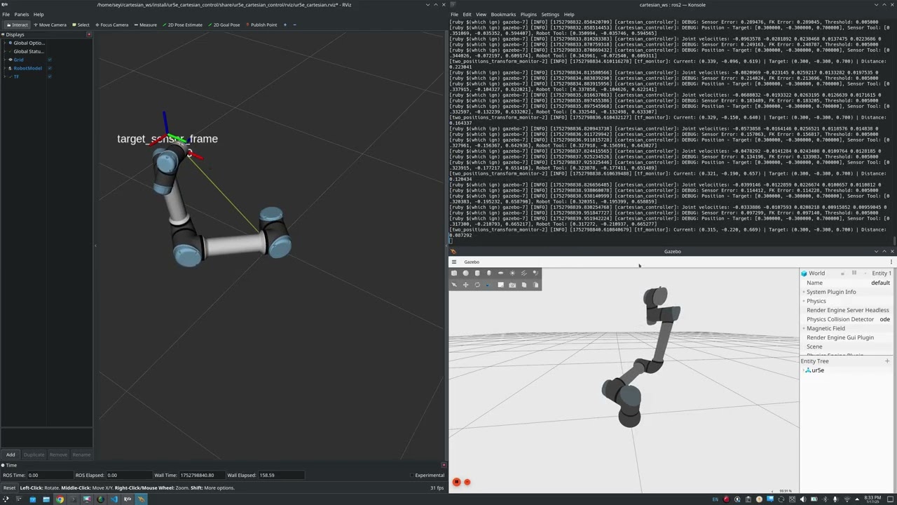
Simulation: UR5e tracking dynamic Cartesian targets in Gazebo with RViz visualization overlay.

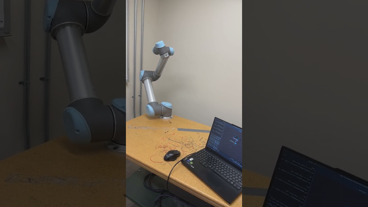
Live Demo: Real UR5 robot executing Cartesian position commands on hardware.

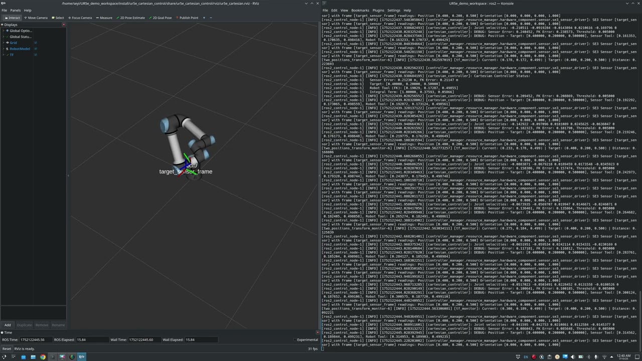
Visualization: TF frames, target tracking, and error convergence in real time.

System Architecture

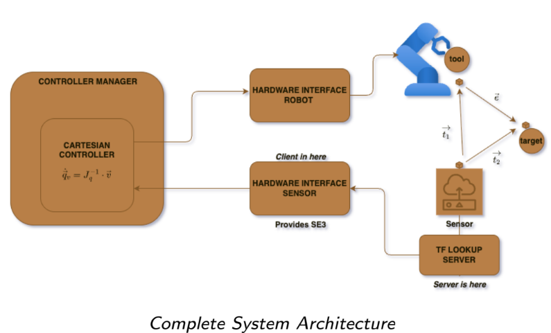
Three ROS 2 packages: se3_sensor_driver (hardware interface reading pose data over TCP), cartesian_controller (PID + Jacobian IK), and ur5e_cartesian_control (launch, config, URDF).

How It Works

Jacobian and Differential Kinematics

The manipulator Jacobian $J(q) \in \mathbb{R}^{6 \times n}$ maps joint velocities to end-effector twist:

\[\begin{bmatrix} \dot{x} \\ \omega \end{bmatrix} = J(q)\,\dot{q}\]

where $\dot{x} \in \mathbb{R}^3$ is the linear velocity, $\omega \in \mathbb{R}^3$ is the angular velocity, $q \in \mathbb{R}^n$ is the joint configuration, and $n = 6$ for the UR5e. Since I only control position (not orientation), I extract the top 3 rows to get the position Jacobian:

\[J_p(q) = J(q)_{[1:3,\,:]} \;\in\; \mathbb{R}^{3 \times 6}\]

The velocity-level inverse kinematics problem is then:

\[\dot{q} = J_p^{\dagger}\,\dot{x}_{\text{cmd}}\]

where $J_p^{\dagger}$ is the pseudo-inverse of $J_p$.

SVD-Based Pseudo-Inverse

The standard Moore-Penrose pseudo-inverse is computed via Singular Value Decomposition. Given $J_p = U \Sigma V^T$, where $U \in \mathbb{R}^{3 \times 3}$, $\Sigma = \text{diag}(\sigma_1, \sigma_2, \sigma_3)$, and $V \in \mathbb{R}^{6 \times 3}$:

\[J_p^{\dagger} = V \Sigma^{-1} U^T\]

The problem is that near singular configurations, some $\sigma_i \to 0$, and $\sigma_i^{-1} \to \infty$. This produces unbounded joint velocities that are physically dangerous.

Tikhonov Regularization (Damped Least Squares)

Instead of the standard pseudo-inverse, I use Tikhonov regularization. This replaces the exact inverse with a damped version by adding a regularization term $\lambda$ (the damping factor):

\[J_p^{*} = V \Sigma^{*} U^T\]

where each regularized singular value is:

\[\sigma_i^{*} = \frac{\sigma_i}{\sigma_i^2 + \lambda^2}\]

This is equivalent to solving the damped least squares problem:

\[\dot{q} = \arg\min_{\dot{q}} \left\| J_p \dot{q} - \dot{x}_{\text{cmd}} \right\|^2 + \lambda^2 \left\| \dot{q} \right\|^2\]

The closed-form solution is:

\[\dot{q} = J_p^T \left( J_p J_p^T + \lambda^2 I \right)^{-1} \dot{x}_{\text{cmd}}\]

When $\sigma_i \gg \lambda$, the regularized inverse behaves like the standard pseudo-inverse. When $\sigma_i \to 0$, the damping term dominates, and $\sigma_i^{*} \to 0$ smoothly instead of blowing up. In practice, the arm gracefully slows down near singularities instead of generating unbounded joint velocities. I use $\lambda = 0.05$.

PID Control Law

The Cartesian position error drives a full PID controller. Given the current end-effector position $x(t)$ and the target $x_d(t)$, the position error is:

\[e(t) = x_d(t) - x(t) \;\in\; \mathbb{R}^3\]

The PID control law computes the commanded Cartesian velocity:

\[\dot{x}_{\text{cmd}}(t) = K_p\, e(t) + K_i \int_0^t e(\tau)\,d\tau + K_d\, \frac{de(t)}{dt}\]

where $K_p, K_i, K_d \in \mathbb{R}^{3 \times 3}$ are diagonal gain matrices (one gain per axis). In discrete time with timestep $\Delta t$:

\[\dot{x}_{\text{cmd}}[k] = K_p\, e[k] \;+\; K_i \sum_{j=0}^{k} e[j]\,\Delta t \;+\; K_d\, \frac{e[k] - e[k-1]}{\Delta t}\]

Anti-Windup

The integral term can accumulate unbounded error when the robot is physically blocked or the target is unreachable. I clamp the integral per axis:

\[\left| \int e_i(\tau)\,d\tau \right| \leq L_{\text{max}}\]

where $L_{\text{max}} = 1.0$ m-s. If the accumulated integral exceeds this bound, it is saturated to $\pm L_{\text{max}}$.

Full Control Pipeline

Combining everything, the complete pipeline at each 500Hz timestep is:

\[e[k] = x_d - x[k]\] \[\dot{x}_{\text{cmd}}[k] = K_p\, e[k] + K_i\, \text{clamp}\!\left(\textstyle\sum e \Delta t\right) + K_d\, \dot{e}[k]\] \[J_p = U \Sigma V^T \quad\text{(KDL Jacobian + SVD)}\] \[\dot{q}_{\text{cmd}} = \alpha \cdot V \Sigma^{*} U^T \, \dot{x}_{\text{cmd}}\]

where $\alpha = 0.07$ is the velocity scaling factor that limits maximum joint speeds for safety.

Tuned Parameters

Parameter	Symbol	Value
Proportional gain	$K_p$	diag(2.2, 2.2, 2.2)
Integral gain	$K_i$	diag(0.02, 0.02, 0.02)
Derivative gain	$K_d$	diag(0.5, 0.5, 0.5)
Damping factor	$\lambda$	0.05
Velocity scaling	$\alpha$	0.07
Integral clamp	$L_{\text{max}}$	1.0
Control rate		500 Hz

Results

Metric	Value
Control loop rate	500 Hz
Position accuracy	±0.7 mm
Convergence time	< 3 sec (50cm moves)
Workspace	Full UR5e envelope
Singularity behavior	Graceful slowdown via Tikhonov damping

Links

View on GitHub

Simulation Demo

Live Demo

RViz Visualization