Fixed-Wing UAV Autopilot & State Estimation

Complete fixed-wing UAV autopilot built from first principles. Successive loop closure PID architecture, dual EKFs for attitude and GPS smoothing, wind disturbance rejection, and closed-loop waypoint tracking validated in nonlinear 6DOF Simulink simulation. Every Jacobian derived by hand.

Live Demo

Fixed-Wing UAV Autopilot & State Estimation

Overview

I built a complete autopilot and state estimation system for a fixed-wing UAV from first principles. No off-the-shelf autopilot stacks, no borrowed controllers. Every transfer function, every Jacobian, every covariance matrix – derived by hand, implemented in MATLAB/Simulink, and validated against a nonlinear 6DOF simulation under wind disturbances.

The core of the project is two Extended Kalman Filters running in parallel: one fusing gyro and accelerometer data to estimate attitude, the other smoothing 1Hz GPS measurements into continuous position/velocity estimates using accelerometer-propagated velocity. Both feed into a successive loop closure PID autopilot that tracks waypoints in gusting wind.

Demo

Simulink Architecture

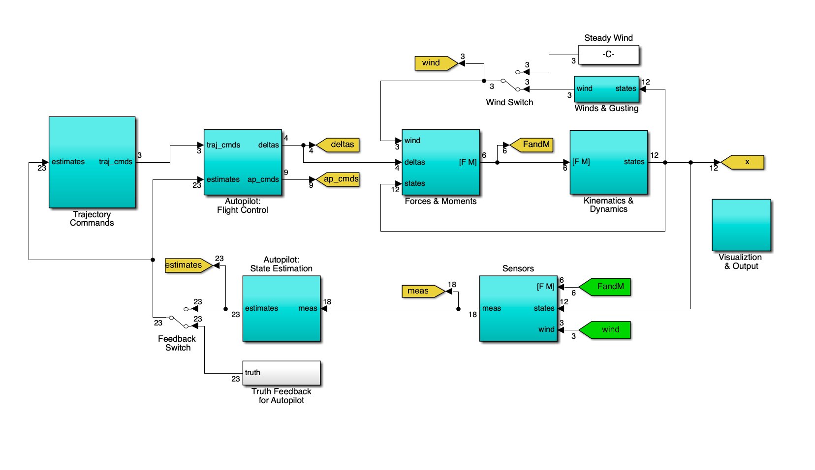
Full Simulink block diagram. Six subsystems in a closed feedback loop: trajectory commands, flight control, forces & moments, kinematics & dynamics, sensors, and state estimation. The feedback switch lets me toggle between truth and estimated states for systematic validation.

Six major subsystems:

Trajectory Commands – waypoint-based reference signals for altitude, airspeed, and heading
Autopilot: Flight Control – nested PID controllers producing 4 control surface deflections ($\delta_e, \delta_a, \delta_r, \delta_t$)
Forces & Moments – aerodynamic forces and propulsion from control inputs, wind, and current state
Kinematics & Dynamics – full nonlinear 6DOF equations of motion (12 states)
Sensors – noisy gyro, accelerometer, GPS (1Hz), barometer, magnetometer, pitot tube
Autopilot: State Estimation – dual EKFs feeding clean estimates back to the controller

Control Architecture

The autopilot uses successive loop closure with bandwidth separation. Fast inner loops handle attitude, slower outer loops handle trajectory.

Inner Loops (Attitude)

**Pitch:** PID with rate feedback commands $$\delta_e$$ from pitch error. **Roll:** PID commands $$\delta_a$$ from roll error, with roll-rate gyro feedback for damping. Both have anti-windup. Tuned by checking gain and phase margins at each stage.

Outer Loops (Trajectory)

**Altitude hold:** Commands $$\theta_c$$ from altitude error. Bandwidth separated from pitch inner loop by 5x+. **Airspeed hold:** Commands throttle $$\delta_t$$ from airspeed error. **Course hold:** Commands $$\phi_c$$ from heading error, with crosswind compensation and crab angle correction.

Attitude EKF

The attitude EKF estimates roll ($\phi$) and pitch ($\theta$) by fusing gyroscope measurements (prediction) with accelerometer measurements (correction). I derived every matrix by hand.

State Vector and Euler Angle Kinematics

$$\hat{x}_{\text{att}} = \begin{bmatrix} \phi \\ \theta \end{bmatrix}, \quad f_{\text{att}} = \begin{bmatrix} p + q\sin\phi\tan\theta + r\cos\phi\tan\theta \\ q\cos\phi - r\sin\phi \end{bmatrix}$$ where $$p, q, r$$ are raw gyroscope measurements (body-frame angular rates).

A Matrix (2x2 Dynamics Jacobian)

$$A_{\text{att}} = \begin{bmatrix} q\cos\phi\tan\theta - r\sin\phi\tan\theta & (r\cos\phi + q\sin\phi)\sec^2\theta \\[4pt] -r\cos\phi - q\sin\phi & 0 \end{bmatrix}$$

Measurement Model (Accelerometer)

The accelerometer measures the gravity vector resolved into the body frame plus centripetal terms (assuming translational dynamics are much slower than rotational): $$h_{\text{att}} = \begin{bmatrix} q\hat{V}_a\sin\theta + g\sin\theta \\[4pt] r\hat{V}_a\cos\theta - p\hat{V}_a\sin\theta - g\cos\theta\sin\phi \\[4pt] -q\hat{V}_a\cos\theta - g\cos\theta\cos\phi \end{bmatrix}$$

C Matrix (3x2 Measurement Jacobian)

$$C_{\text{att}} = \begin{bmatrix} 0 & g\cos\theta + \hat{V}_a q\cos\theta \\[4pt] -g\cos\phi\cos\theta & g\sin\phi\sin\theta - \hat{V}_a r\sin\theta - \hat{V}_a p\cos\theta \\[4pt] g\cos\theta\sin\phi & \hat{V}_a q\sin\theta + g\cos\phi\sin\theta \end{bmatrix}$$

Noise Tuning

For process noise, I used gyro noise variance directly since it maps one-to-one to attitude rate error:

\[Q = \begin{bmatrix} \sigma_{\text{gyro}}^2 & 0 \\ 0 & \sigma_{\text{gyro}}^2 \end{bmatrix}\]

The measurement noise was the tricky part. The raw accelerometer noise variance ($\sigma^2_{\text{accel}} = 6.02 \times 10^{-4}$ m$^2$/s$^4$) is way too small because the measurement model ignores aerodynamic effects and other real-world dynamics. I had to scale R by $10^{4.5}$:

\[R = 10^{4.5} \times \begin{bmatrix} \sigma_{\text{accel}}^2 & 0 & 0 \\ 0 & \sigma_{\text{accel}}^2 & 0 \\ 0 & 0 & \sigma_{\text{accel}}^2 \end{bmatrix}\]

This tells the EKF: trust the gyro-based prediction more than the accelerometer correction. The bigger R compensates for all the modeling simplifications in the measurement model. I use 10 sub-steps per sample period for numerical stability, symmetrize the covariance after each update, and wrap the state to $[-\pi, \pi]$.

GPS Smoother EKF

1Hz GPS is too slow for flight control. Raw updates create discrete jumps in position and velocity, causing stepped responses in heading and altitude tracking. I built a 6-state EKF that propagates between GPS fixes using accelerometer data rotated into the NED frame.

State Vector and Propagated Velocity Model

$$\hat{x}_{\text{gps}} = \begin{bmatrix} \hat{p}_n \\ \hat{p}_e \\ \hat{p}_d \\ \hat{v}_n \\ \hat{v}_e \\ \hat{v}_d \end{bmatrix}_{6 \times 1}, \quad f(\hat{x}, u) = \begin{bmatrix} \hat{v}_n \\ \hat{v}_e \\ \hat{v}_d \\ a_n^{\text{NED}} \\ a_e^{\text{NED}} \\ a_d^{\text{NED}} \end{bmatrix}$$ The NED-frame acceleration comes from body-frame accelerometer readings rotated by the attitude estimate and compensated for gravity: $$\mathbf{a}^{\text{NED}} = (R_b^{\text{NED}})^\top \begin{bmatrix} a_x \\ a_y \\ a_z \end{bmatrix} + \begin{bmatrix} 0 \\ 0 \\ g \end{bmatrix}$$ This is the key idea: rather than assuming constant velocity between GPS fixes, I integrate accelerometer readings to propagate velocity at the full sensor rate. No more discrete jumps.

A and C Matrices

Position derivative equals velocity, velocity derivative equals acceleration (enters as input, not state). Clean structure: $$A = \begin{bmatrix} 0_{3\times3} & I_{3\times3} \\ 0_{3\times3} & 0_{3\times3} \end{bmatrix}_{6\times6}, \quad C = I_{6\times6}$$ GPS corrections only fire when a new measurement arrives (~every 100 iterations). I detect this by comparing current $$p_n, p_e$$ against stored previous values.

Closing the Loop

The final system feeds all state estimates back to the autopilot:

State	Source
$\phi, \theta$	Attitude EKF
$\psi$	Filtered magnetometer
$p, q, r$	Filtered gyroscopes
$h$	Barometric altimeter
$V_a$	Pitot tube
Position, velocity	GPS Smoother EKF

With the feedback switch set to estimates instead of truth, the UAV is simultaneously learning its attitude AND regulating flight commands. The first 10-15 seconds show transient oscillations as the attitude EKF converges, then the controller tracks waypoints smoothly.

Results

I validated the complete system over 200-second runs with gusting winds:

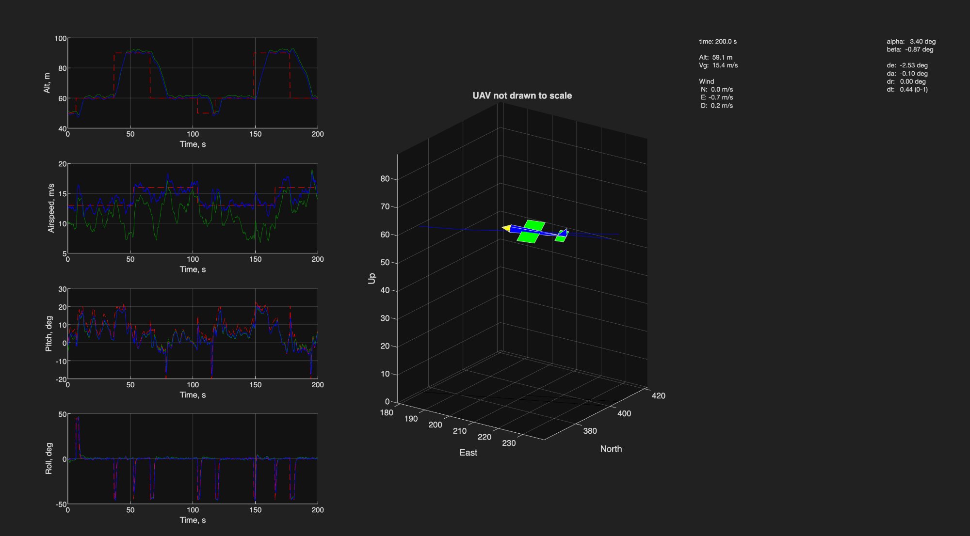
200-second closed-loop simulation with gusting winds and state estimate feedback. Left: altitude, airspeed, pitch, and roll tracking (red = command, blue = estimate, green = truth). Right: 3D waypoint trajectory.

Detailed flight data: altitude hold between 60-90m, airspeed regulation around 15 m/s, pitch and roll tracking under wind disturbance.

Attitude estimation: Roll and pitch errors within +/-5 degrees (1-sigma), consistent with $P_0$
GPS smoothing: Sub-2m position error variation with smooth curvature between 1Hz measurements
Wind rejection: Stable flight under steady wind and gusting conditions with crosswind compensation
Estimator feedback: Minimal performance degradation switching from truth to estimated feedback

Code Files

Attitude EKF (Roll & Pitch Estimator)

matlab

%%%%%%%%%%%%%%%%%%%%%%%%%%%%%%%%%%%%%%%%%%%%%%%%%%%%%%%%%%
% Attitude EKF - Estimate roll (phi) and pitch (theta)
% from gyroscope prediction + accelerometer correction
%%%%%%%%%%%%%%%%%%%%%%%%%%%%%%%%%%%%%%%%%%%%%%%%%%%%%%%%%%

% Q matrix - process noise from gyro
Q_att = diag([P.sigma_noise_gyro^2, P.sigma_noise_gyro^2]);

% R matrix - measurement noise from accel, scaled by 10^m
m = 4.5;
R_att = 10^m * diag([P.sigma_noise_accel^2, ...
        P.sigma_noise_accel^2, P.sigma_noise_accel^2]);

persistent xhat_att P_att
if(time == 0)
    xhat_att = [0; 0];  % [phi; theta] - start level
    P_att = diag([5*pi/180, 5*pi/180].^2);  % +/-5 deg
end

% === PREDICTION (N sub-steps) ===
N = 10;
for i = 1:N
    % State dynamics: Euler angle kinematics
    f_att = [p_gyro + q_gyro*sin(xhat_att(1))*tan(xhat_att(2)) ...
             + r_gyro*cos(xhat_att(1))*tan(xhat_att(2));
             q_gyro*cos(xhat_att(1)) - r_gyro*sin(xhat_att(1))];

    % Jacobian A
    A_att = getAjacobian(xhat_att, [p_gyro q_gyro r_gyro]);

    % Propagate state and covariance
    xhat_att = xhat_att + (P.Ts/N) * f_att;
    P_att = P_att + (P.Ts/N)*(A_att*P_att + P_att*A_att' + Q_att);
    P_att = real(0.5*P_att + 0.5*P_att');
end

% === MEASUREMENT UPDATE ===
y_att = [ax_accel; ay_accel; az_accel];

h_att = [q_gyro*Va_hat*sin(xhat_att(2)) + P.gravity*sin(xhat_att(2));
         r_gyro*Va_hat*cos(xhat_att(2)) ...
         - p_gyro*Va_hat*sin(xhat_att(2)) ...
         - P.gravity*cos(xhat_att(2))*sin(xhat_att(1));
         -q_gyro*Va_hat*cos(xhat_att(2)) ...
         - P.gravity*cos(xhat_att(2))*cos(xhat_att(1))];

C_att = getCjacobian(xhat_att, [p_gyro q_gyro r_gyro Va_hat]);

% Kalman gain and correction
L_att = P_att*C_att'/(C_att*P_att*C_att' + R_att);
xhat_att = xhat_att + L_att*(y_att - h_att);
P_att = (eye(2) - L_att*C_att)*P_att;
xhat_att = mod(xhat_att + pi, 2*pi) - pi;

GPS Smoother EKF (Propagated Velocity Model)

matlab

%%%%%%%%%%%%%%%%%%%%%%%%%%%%%%%%%%%%%%%%%%%%%%%%%%%%%%%%%%
% GPS Smoother EKF - 6-state position/velocity estimator
% Uses accelerometer-propagated velocity between 1Hz GPS
%%%%%%%%%%%%%%%%%%%%%%%%%%%%%%%%%%%%%%%%%%%%%%%%%%%%%%%%%%

persistent xhat_gps P_gps pn_gps_prev pe_gps_prev

if (time == 0)
    xhat_gps = [pn_gps; pe_gps; -alt_gps; ...
                Vn_gps; Ve_gps; Vd_gps];
    P_gps = diag([2^2, 2^2, 2^2, 0.5^2, 0.5^2, 0.5^2]);
    pn_gps_prev = pn_gps;
    pe_gps_prev = pe_gps;
end

% Detect new GPS measurement
new_gps = (pn_gps ~= pn_gps_prev || pe_gps ~= pe_gps_prev);

% Body-to-NED rotation + gravity compensation
Rb_ned = eulerToRotationMatrix(phi_hat, theta_hat, psi_hat)';
accel_ned = Rb_ned * [ax_accel; ay_accel; az_accel] + [0; 0; P.gravity];

% System matrices
A = [zeros(3,3), eye(3); zeros(3,3), zeros(3,3)];
Q = diag([0.1^2, 0.1^2, 0.1^2, 0.2^2, 0.2^2, 0.2^2]);

% === PROPAGATE with accel-based velocity model ===
xhat_gps = xhat_gps + P.Ts * [xhat_gps(4:6); accel_ned];
P_gps = P_gps + P.Ts * (A*P_gps + P_gps*A' + Q);

% === CORRECT at 1Hz GPS rate ===
if new_gps
    C = eye(6);
    R = diag([2 2 2 0.1 0.1 0.1].^2);
    y = [pn_gps; pe_gps; -alt_gps; Vn_gps; Ve_gps; Vd_gps];
    
    L = P_gps*C'/(C*P_gps*C' + R);
    xhat_gps = xhat_gps + L*(y - xhat_gps);
    P_gps = (eye(6) - L*C)*P_gps;
    P_gps = (P_gps + P_gps')/2;
    
    pn_gps_prev = pn_gps;
    pe_gps_prev = pe_gps;
end

Jacobian Helper Functions

matlab

% A Jacobian for attitude EKF (2x2)
function A = getAjacobian(xhat_att, gyro)
    phi = xhat_att(1); theta = xhat_att(2);
    p = gyro(1); q = gyro(2); r = gyro(3);
    A = [q*cos(phi)*tan(theta) - r*sin(phi)*tan(theta), ...
         (r*cos(phi) + q*sin(phi))*(sec(theta))^2;
         -r*cos(phi) - q*sin(phi), 0];
end

% C Jacobian for attitude EKF (3x2)
function C = getCjacobian(xhat_att, inputs)
    phi = xhat_att(1); theta = xhat_att(2);
    p = inputs(1); q = inputs(2);
    r = inputs(3); Va = inputs(4);
    g = 9.81;
    C = [0, g*cos(theta) + Va*q*cos(theta);
         -g*cos(phi)*cos(theta), ...
         g*sin(phi)*sin(theta) - Va*r*sin(theta) - Va*p*cos(theta);
         g*cos(theta)*sin(phi), ...
         Va*q*sin(theta) + g*cos(phi)*sin(theta)];
end

Demo

Controls Flight MATLAB State-Estimation

State	Source
\(\phi, \theta\)	Attitude EKF
\(\psi\)	Filtered magnetometer
\(p, q, r\)	Filtered gyroscopes
\(h\)	Barometric altimeter
\(V_a\)	Pitot tube
Position, velocity	GPS Smoother EKF